The Underlying Intuition of Wav2Vec2's CNN

An Introduction

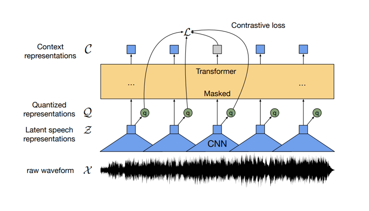
Typically, every explanation of the Wav2vec2 architecture begins with the iconic diagram, but without extensive background, it is hard to know what the cones labeled as the CNN are really doing. What does it actually mean to extract features from audio? Let's find a stronger visual intuition for this.

Background

For those new to audio processing, audio is incredibly dense compared to other forms of data like text.

You can imagine sound as a continuous, smooth curve, but because we want to discretize this (represent audio numerically), we take snapshots of this wave at regular intervals. How frequently we take these snapshots in one second of sound is the sampling rate. This sampling rate decides how much information we have to store in audio.

The typical sampling rate of 16kHz represents processing 16 thousands values per second of audio. That's a lot of information! So how can the Wav2Vec2 architecture handle all of this information?

The Feature Extractor

The Feature Extractor, also called the Convolutional Neural Network (CNN), aims to extract high-level features while compressing a very dense temporal dimension . Think of it as when you want to do a quick portrait of someone: you want to capture their distinguishable facial features without spending too much time capturing every detail.

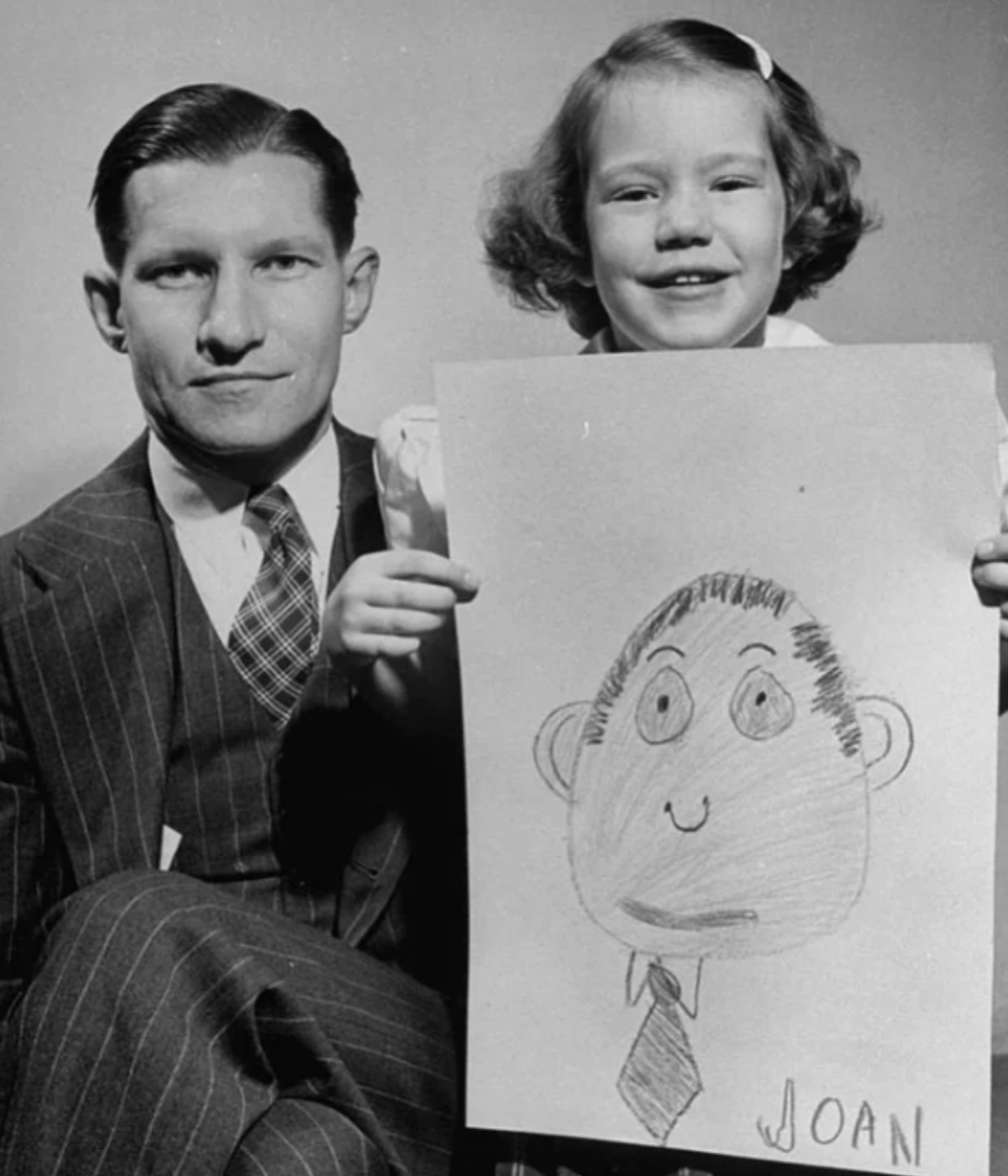
Kids asked to draw their fathers in 1949

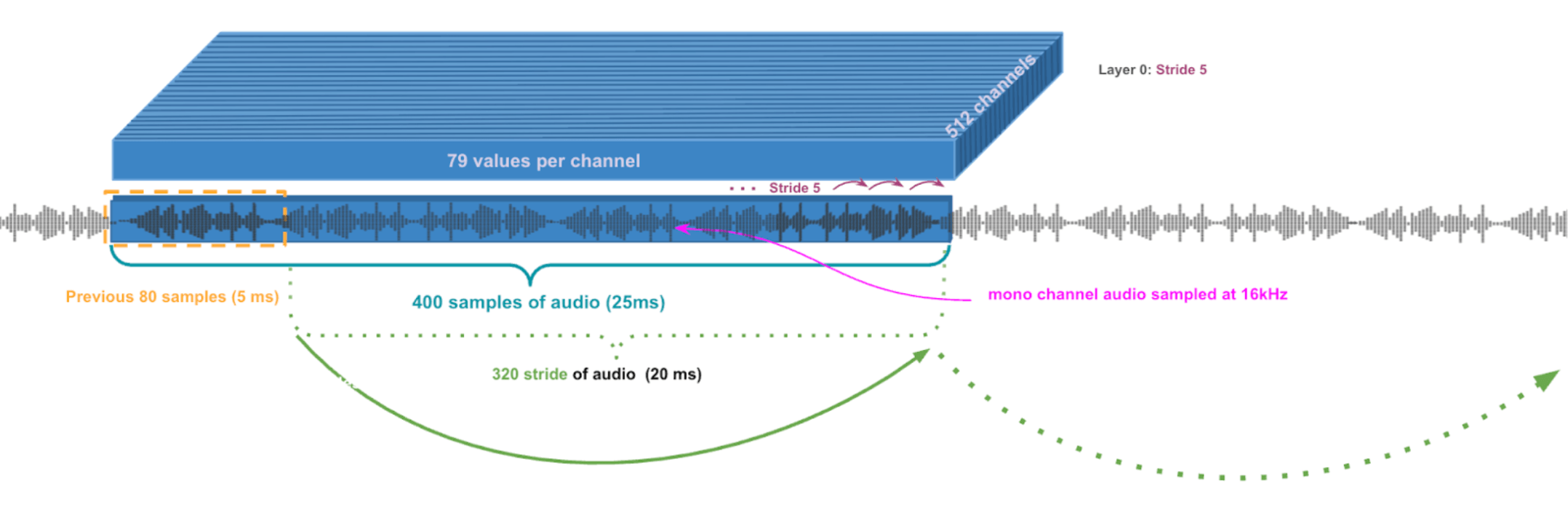
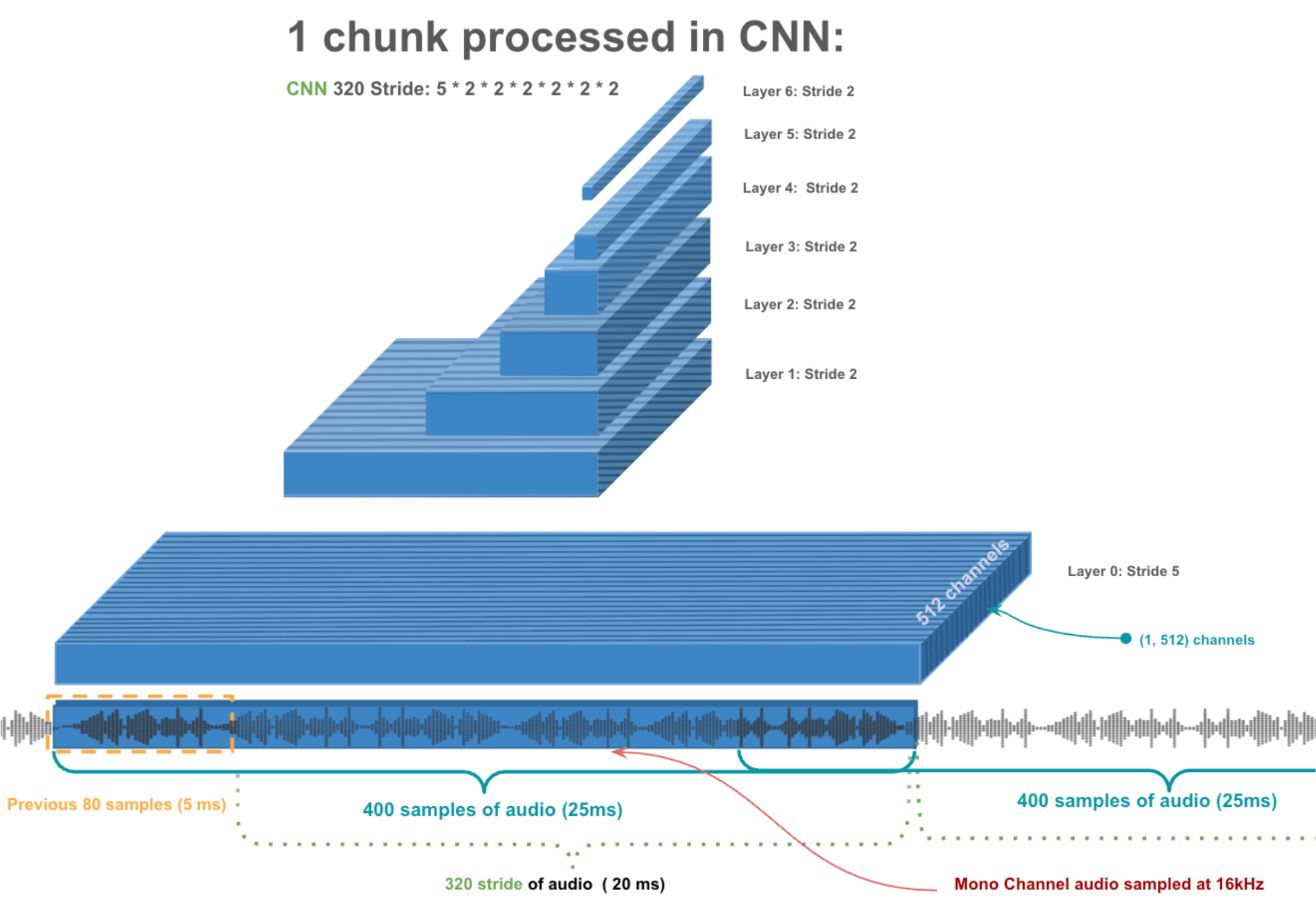
The Feature Extractor will take 1/50th of a second (20ms) at a time and use the previous 1/200th of a second (5ms) to give itself some context. So lets take a closer look at how that single 25ms chunk gets processed.

Audio Stream to Representation

This first 25ms chunk of raw audio starts as a chunk of 400 values (seconds × sampling-rate = 0.025 × 16,000 = 400 samples) representing the audio waveform. Just a simple list like

[0.1, -0.3, 0.8, -0.2, 0.1, 0.5, -0.1, -0.4, 0.2, 0.3, ...]

Think of an audio waveform representing tiny vibrations of air molecules that result in changes in air pressure. While very cool, air pressure changes do not communicate any clear patterns in acoustic signals like pitch, timbre, and other audio characteristics. It would be much better to transform these 400 temporal samples into 512 higher-level features that capture these different acoustic properties across the entire 25ms window.

So that's what the feature extractor does, starting with the first layer. It takes this single monochannel audio input and projects to 512 dimensional space via 512 channels. And to load each of these channels, we look at a 1 × 10 window and take the dot product against a 10 × 1 kernel to compute a single value. We then slide over by a stride of 5 samples for the next 1 × 10 window. After the first window processes 10 unseen samples, the remaining 1 × 10 windows process 5 seen + 5 unseen samples at a time. So to find how many windows span the 400 samples, we consider just what are the unseen samples: 78 windows process 5 unseen samples at a time and the very first window processes 10 unseen samples, giving us 79 windows for this layer.

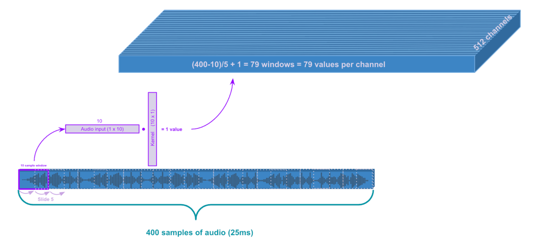
First layer convolution: kernel_size = 10, stride = 5

The output dimension should feel intuitive but if you don't want to use your brain to figure out your output dimension of a single channel you can use this nice formula:

# Layer 0
kernel_size = 10
stride = 5
input_values = 400
num_output_values = math.floor((input_values - kernel_size) / stride) + 1  # 79

Okay, now we have our first layer!

First Layer Convolution

Remember, we want to reduce the temporal dimension, so let's apply another convolution! To do this, the next layer will stride every second value of a 3-sample-window of the first layer. So basically look at every second value. Can you guess what the next block will look like?

Using our little formula…

# Layer 1
kernel_size = 3
stride = 2
input_values = 79
math.floor((input_values - kernel_size) / stride + 1)  # Output = 39

39 values across 512 channels, nice! Layers 1–4 have the same kernel size and stride so lets just repeat this…

kernel_size = 3
stride = 2
input_values = 79  # Layer 0 input

# Layers 1-4
for i in range(4):
    output = math.floor((input_values - kernel_size) / stride + 1)
    input_values = output
# output = 39 -> 19 -> 9 -> 4

Awesome! Now the last 2 layers have stride and kernel size 2..

kernel_size = 1
stride = 2
input_values = 4  # Layer 4 input

# Layers 5-6
for i in range(2):
    output = math.floor((input_values - kernel_size) / stride + 1)
    input_values = output
# output = 2 -> 1

Wow. We now just have a single value across 512 channels.

Throughout this process, activation functions like GeLU add non-linearity between each layer, allowing the network to learn complex patterns.

Single Chunk Processed by CNN

Why not just directly compress from 400 samples to 512 features in one step?

Jumping directly would require learning 204,800 parameters in one massive linear transformation, which is both hard to optimize and limited in what patterns it can capture. Multiple smaller layers with non-linear activations between them train more reliably and can build complex representations by combining simpler patterns. A chef that takes time to make components of a dish from scratch will produce a much better, complex dish than any microwave meal.

So that's how we process a single 25ms chunk of audio - transforming 400 raw samples into a rich 512-dimensional feature vector. Now we slide this entire process across the audio stream, moving 320 samples at a time...

All of that has been nicely wrapped in a few lines of code:

input_values = inputs.input_values.type(torch.float32)
with torch.no_grad():
    extract_features = model.wav2vec2.feature_extractor(input_values)

We can also grab the attention masks to

attention_mask = inputs.attention_mask
with torch.no_grad():
    extract_features = model.wav2vec2.feature_extractor(input_values).transpose(1, 2)
    attention_masks = model.wav2vec2._get_feature_vector_attention_mask(
        extract_features.shape[1], 
        attention_mask, 
        add_adapter=False
    )

Feature Projection

Okay we are almost done, the Transformer (yellow block of the first Diagram) just requires a much larger dimension input. So we will just apply a linear projection to reach 1024 features. Lastly, we make sure to mask out the features we don't care about by using the attention masks.

hidden_states, _ = model.wav2vec2.feature_projection(extract_features)
hidden_states = model.wav2vec2._mask_hidden_states(hidden_states, attention_masks)

We did it! 🎉 You just walked through exactly what the feature extractor (CNN) does in the Wav2Vec2 architecture!

Takeaways

After walking through each convolutional layer, you can probably understand how much computation and time this can consume. To be able to get these audio models to run in real time requires some careful optimization which is critical for many of our products. Learn more about streaming optimizations here!

Part 2: The Transformer!